F# and linear regression

Recently, we implemented a simple example in F# illustrating the use of Gradient Descent to find the minimum of a chosen function. Today, we will use the experience gained for something more practical – predicting salary based on experience.

Data

We will use a publicly available, simple dataset containing fictional data, which, due to its simplicity, will facilitate understanding of the topic:

https://www.kaggle.com/datasets/abhishek14398/salary-dataset-simple-linear-regression

Although we will use fictional data, the method of building a predictive model will be as realistic as possible.

Type Providers

The data is available in the form of a csv file, which will be an excuse to use a convenient tool of the F# language – type providers. In this specific case, it will be CsvProvider, available in the FSharp.Data library.

CsvProvider allows generating F# types based on the data structure in csv files. This way, we won’t have to manually define data types in F# code, and we’ll benefit from strong, static typing in F#.

In our case, the data file contains a list of observations described by the following features:

• Index – ordinal number, irrelevant from our point of view
• YearsExperience – experience measured in years
• Salary – salary

To define a type for the examined dataset and a single observation, the following line is enough:

type Data = CsvProvider<"salary_dataset.csv", ResolutionFolder=__SOURCE_DIRECTORY__>
type Observation = Data.Row

Now all we need to do is load the data from the file and transform it into a collection of observations:

let data = Data.Load(__SOURCE_DIRECTORY__ + "/salary_dataset.csv")
let observations = data.Rows

Using strong typing, we can easily refer to individual features of the observations:

observations
|> Seq.iter (fun o -> printfn $"%.1f{o.YearsExperience} -> %.2f{o.Salary}")

Each of the observations has defined features with names consistent with the header of the csv file, and importantly, with an assigned type (in this case, decimal). It is exactly as if we had previously defined this type ourselves, parsed the file, and built a collection of records from it.

Observations

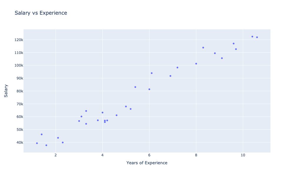
Let’s try to visualize the studied set of observations.

We will start with a helper function responsible for formatting and displaying charts:

let showChart (charts: GenericChart seq) =
    charts
    |> Chart.combine
    |> Chart.withSize (1000., 600.)
    |> Chart.withTitle "Salary vs Experience"
    |> Chart.withXAxisStyle ("Years of Experience")
    |> Chart.withYAxisStyle ("Salary")
    |> Chart.show

Now let’s define a chart presenting the studied observations and try to display it:

let observationsChart =
    observations
    |> Seq.map (fun o -> o.YearsExperience, o.Salary)
    |> Chart.Point
    |> Chart.withTraceInfo ("Observations")

showChart [ observationsChart ]

On the chart, we can see the dependency of salary level on experience. With the naked eye, we can observe a strong visible relationship between salary and experience. We can express such a dependency numerically, in the form of a so-called correlation coefficient.

We can implement our own function using the formula:

r = Σ((xi – x̄)(yi – ȳ)) / √(Σ(xi – x̄)² * Σ(yi – ȳ)²)

Where:

• xi and yi are individual values of variables X and Y
• x̄ and ȳ are the mean values of variables X and Y
• Σ denotes summation over all observations (i = 1, 2, …, n)
• n is the number of observations

For simplicity, we will use another great library: Fsharp.Stats

observations
|> pearsonBy (fun o -> o.YearsExperience, o.Salary)
|> printfn "Pearson correlation: %.2f"

Either way, we will obtain a result of 0.98, which indicates a very strong positive correlation (both features increase proportionally). A result close to zero would indicate a lack of correlation between the features, while a result close to -1 would indicate a strong negative correlation (an increase in one feature causes a proportional decrease in the other).

Domain modeling

Our goal will be to implement a model that will predict the salary as effectively as possible for a given experience.

Let’s start by defining the problem domain:

type Experience = decimal

type Salary = float

type Model = Experience -> Salary

Domain-Driven Design purists would be delighted 😉

Baseline model

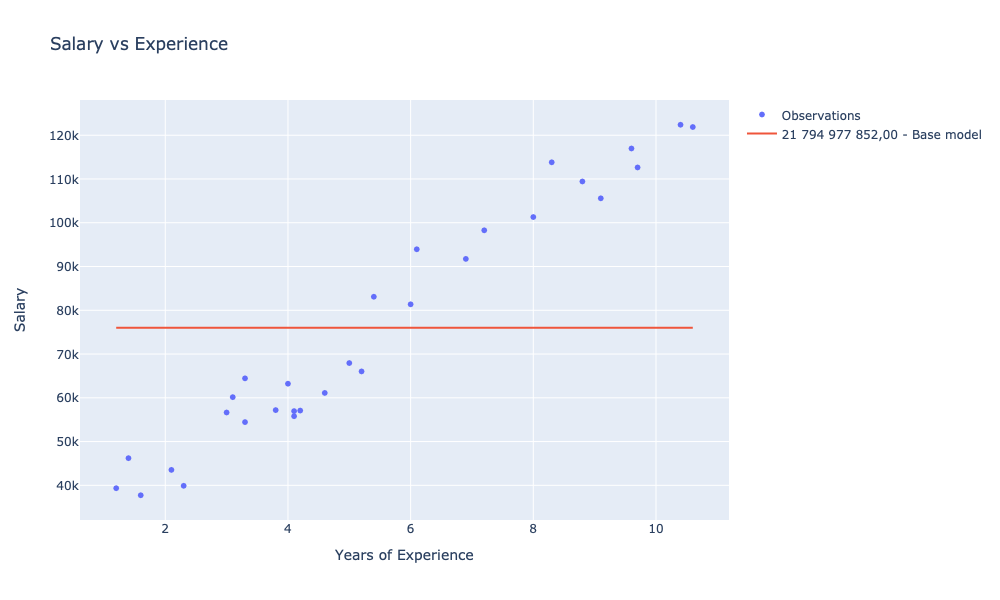
Now, to have something to refer to, let’s define a simple and naive model. Let’s assume that this model will return the average salary regardless of experience:

let averageModel (experience: Experience) =
    observations |> Seq.averageBy (fun o -> o.Salary) |> float

In order to compare future models to this baseline, we need some method of evaluating the model’s effectiveness. We need to determine a quality metric:

Sum of Squared Errors

We will use the so-called Sum of Squared Errors (SSE), which is the difference between the predicted and actual values. Let’s start with the formula:

SSE = Σ(yi – ŷi)²

Where:

• yi is the actual value of the i-th observation,
• ŷi is the predicted value of the i-th observation,
• Σ denotes summation over all observations (i = 1, 2, …, n),
• n is the number of observations.

let sse (obs: Observation seq) (model: Model) =
    obs
    |> Seq.sumBy (fun o -> (model o.YearsExperience - float o.Salary) ** 2.0)

Now we can evaluate our baseline model:

let avgModelScore = sse observations averageModel

Then define a chart for it:

let scoreFormat = "N2"

let avgModelChart =
    observations
    |> Seq.map (fun o -> o.YearsExperience, averageModel o.YearsExperience)
    |> Chart.Line
    |> Chart.withTraceInfo $"%s{avgModelScore.ToString(scoreFormat)} - Base model"

showChart [ observationsChart; avgModelChart ]

Linear regression

Linear regression is a statistical technique used to analyze the relationship between two variables – the independent variable (in our case, experience) and the dependent variable (in our case, salary). The goal of linear regression is to find the best fit of a straight line to the data, which will allow predicting the value of the dependent variable based on the value of the independent variable.

The formula for a straight line in a two-dimensional space defines the equation:

y = theta1 * x + theta0

where:

• y is the dependent variable
• x is the independent variable
• theta1 is the slope of the line
• theta0 is the intercept

Our task will be to find such theta0 and theta1 for which SSE will be the smallest. We will use the Gradient, described in more detail here. To update the coefficients, we will calculate the partial derivative value for the independent variable separately for each. The derivatives will be computed using various rules, including the chain and power rules.

The function updating the coefficient values may look like this:

let updateThetas (alpha: float) (theta0, theta1) (obs: Observation) =
    let x = float obs.YearsExperience
    let y = float obs.Salary
    let theta0' = theta0 - 2. * alpha * (theta0 + theta1 * x - y)
    let theta1' = theta1 - 2. * alpha * x * (theta0 + theta1 * x - y)
    (theta0', theta1')

For a given observation, we “move” the values of the individual theta coefficients in the negative direction of the gradient – we subtract the value of the derivative multiplied by the learning constant alpha.

Stochastic gradient

We will start with a simpler algorithm – the stochastic gradient, which allows for faster and more efficient optimization of the error function. In the case of the stochastic gradient, the calculation of the error function gradient is performed only for a single training example in each iteration of the algorithm. In this way, this algorithm is more effective for large datasets, as it requires less computation and is not dependent on the entire dataset.

The advantage of the stochastic gradient is its speed and ability to achieve good results for a large number of training data. However, the disadvantage is that the algorithm is more unstable and has a higher probability of reaching a local minimum instead of a global one.

The implementation in F# comes down to:

let stochasticGradient alfa (theta0, theta1) (data: Observation seq) =
    data |> Seq.fold (updateThetas alfa) (theta0, theta1)

We are almost ready to train our first model.

Let’s start with a helper function that builds the Model based on the thetas:

let model (theta0, theta1) (experience: Experience) = float experience * theta1 + theta0

Now we can use all our tools to train the first model:

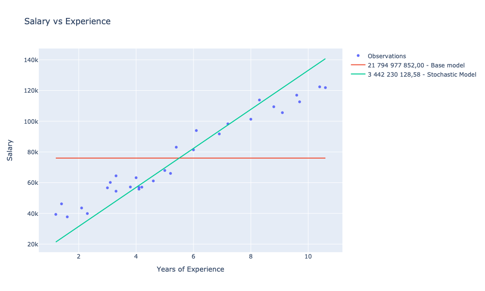
let stochasticModel = stochasticGradient 0.0123 (0., 0.) observations |> model

The value of the learning constant alpha was chosen empirically and should be adjusted each time to the specific problem and dataset.

I encourage you to experiment with different values.

We can evaluate our new model:

let stochasticModelScore = sse observations stochasticModel

and then visualize it:

let stochasticModelChart =
    observations
    |> Seq.map (fun o -> o.YearsExperience, stochasticModel o.YearsExperience)
    |> Chart.Line
    |> Chart.withTraceInfo ($"%s{stochasticModelScore.ToString(scoreFormat)} - Stochastic Model")

showChart [ observationsChart; avgModelChart; stochasticModelChart ]

Batch gradient

This time, for a change, we will update the values of the theta parameters using the entire set of observations in each iteration – hence the name Batch gradient.

Let’s define a function that will implement a single iteration based on the entire set of observations:

let batchUpdateThetas rate (theta0, theta1) (data: Observation seq) =
    let thetas = data |> Seq.map (updateThetas rate (theta0, theta1))

    let theta0' = thetas |> Seq.averageBy fst
    let theta1' = thetas |> Seq.averageBy snd
    (theta0', theta1')

and a function that will search for optimal theta parameters for a specified number of iterations:

let batchEstimation rate iters (data: Observation seq) =
    let rec search (theta0, theta1) i =
        if i = 0 then
            (theta0, theta1)
        else
            search (batchUpdateThetas rate (theta0, theta1) data) (i - 1)

    search (0., 0.) iters

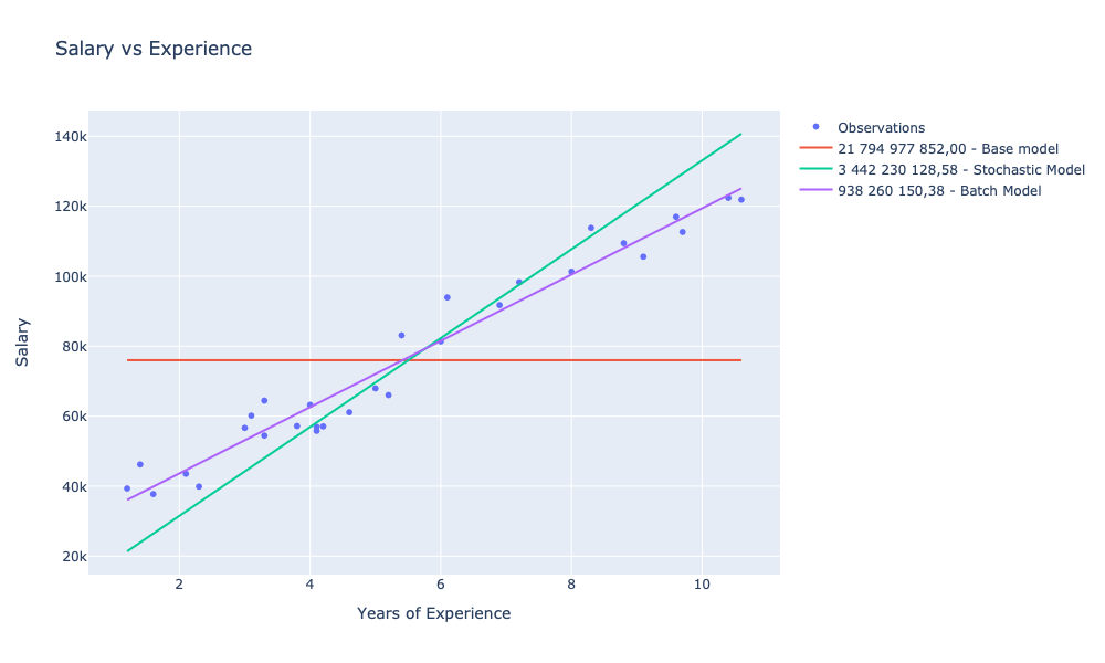
Now we can train another model. Let’s use the same learning constant and 1,000 iterations:

let batchModel = batchEstimation 0.0123 1_000 observations |> model

We can now evaluate and visualize the model:

let batchModelCost = sse observations batchModel

let batchModelChart =
    observations
    |> Seq.map (fun o -> o.YearsExperience, batchModel o.YearsExperience)
    |> Chart.Line
    |> Chart.withTraceInfo $"%s{batchModelCost.ToString(scoreFormat)} - Batch Model"

showChart [
    observationsChart
    avgModelChart
    stochasticModelChart
    batchModelChart
]

Summary

Firstly, F# is a functional programming language that provides flexible tools for data analysis, including linear regression.

In relation to our baseline model, for which SSE was 21,794,977,852.00, we managed to train two models with SSE smaller by:

• 84% (3,442,230,128.58) for stochastic gradient
• 95% (938,260,150.38) for batch gradient

I encourage you to experiment with the number of iterations and learning rate.

It’s also worth noting that in a production approach, we should not train and evaluate the model using the same data. We should ensure that we have a separate training and testing dataset.

Useful links

• F# and Gradient Descent: How to find the minimum of a function in a few minutes?
• FSharp.Data
• FSharp.Stats
• Kaggle
• Residual sum of squares

Complete code

[gist id=”360259b4ae4307372f1516827083649b”]